This applet is designed to provide some intuition into inferential thinking. The goal of the game is to determine the true population mean. There are six game modes, each differentiated by the size of the sample collected. Each game mode has a different true distribution (different population parameters). Each time the user presses the “Simulate Data” button, a new dataset will be generated from the true underlying distribution and the sample mean and sample standard deviation are computed. AFTER you make your guess at the true mean, you can get the truth by selecting the “Get True Mean” button and subsequently hide the truth by selecting the “Hide True Mean” button. DO NOT look at the true mean until you are done with all of the exercises, or you will ruin the game!
7 Introduction to Inference
” A useful property of a test of significance is that it exerts a sobering influence on the type of experimenter who jumps to conclusions on scanty data, and who might otherwise try to make everyone excited about some sensational treatment effect that can well be ascribed to the ordinary variation in his experiment.”
— Gertrude Mary Cox
- Understand conceptually how confidence intervals are constructed
- Know correct interpretation of confidence intervals
- Hypothesis testing null and alternative hypothesis
- Type 1 and type 2 error
- Definition of p-value and how to interpret
7.1 Statistical Inference
It may be helpful at this point to quickly review our goals as statisticians, as well as some of the key concepts that we have covered so far:
First, let’s consider again the primary goal of statistical analysis. We often begin with some population of interest. In particular, we are generally interested in determining some numerical quantity that describes this population. This may include things such as average monthly spending or the proportion of individuals who respond positively to some treatment. As it is typically impractical to measure some quantity within an entire population, we are often limited to collecting a random sample of the population from which we hope to make generalizations that apply to the population as a whole.
The data that we collect is usually random, and we can quantify the amount of uncertainty associated with a particular outcome with a numerical quantity known as a probability. The relationship between possible values of our data and their associated probabilities is known as a probability distribution, two of the most widely used being the normal and binomial distributions, covered in chapter 5.
The act of collecting a sample and computing a statistic is itself a random process and, as such, also follows a probability distribution known as a sampling distribution. As we saw with the Central Limit Theorem introduced in the last chapter, as the number of individuals collected in our sample increases, the computed statistic will increasingly approximate a normal distribution. As with the normal distribution, the sampling distribution will depend on the value of the sample mean, as well as the size of the standard error
Our goal now is to determine how we might use these ideas to go from information in our random sample to statements about the broader population. This process is known as statistical inference and is the focus of the present chapter.
Let’s start by playing a simple “game” in the exercise below.
Exercise 7.1
-
Start with the game mode corresponding to a sample size of 10. Draw at least five samples and record the sample means and sample standard deviations (SD) you observe as in the table below.
Sample Sample mean Sample SD 1 2 3 4 5 - Based on what you have observed in your samples, what do you think is a range of values that would have a good chance of containing the true population mean? How did you select this interval?
- If you could only select one value, what is your best guess for the true population mean? How did you determine your guess?
- Based on what you observed, do you think it is likely or unlikely that the true population mean is -6? Explain your reasoning.
- Now look at the true mean, how close was your best guess? Was the true mean contained in your interval?
-
Repeat exercises (1-5) for each game mode, until you have a range and your best guess of the true mean for all six sample sizes. Determine if the given comparison value for each scenario is likely or unlikely. Summarize your work in the following table.
Sample size Interval Best guess Comparison value Likely/unlikely? Truth 10 -6 30 3 50 0.2 100 70 200 0 500 20 - Were some of the game modes easier than others? Why do you think this was?
- What does the Central Limit Theorem tell us about the variation we would expect in the sample mean as the sample size increases?
How good were you at guessing the truth? To play the game, you had to come up with some method to make your best guess, an interval of plausible values, and finally determine how likely it was that a given value was the truth. These are some of the foundational goals of statistical inference, which help us answer questions like:
- By how much can you expect your blood pressure to be reduced after starting
a blood pressure medication?
- How likely is it that a new cancer treatment will lead to fewer deaths than the current treatment standard?
- After getting the flu, for approximately how many days is someone infectious?
7.2 Point Estimation and Confidence Intervals
The idea of coming up with a single best guess at a population parameter is more formally known as point estimation. For example, using the mean value of a sample to estimate the mean value of the population is a form of point estimation. In other words, it is a single number computed from the sample data that is used to infer the value of the population parameter.
As we have seen in the probability distribution exercises of chapter 5, the process of obtaining a sample is random, which means that sample means computed from two separate samples taken from the same population will likely not be identical. To account for both this random variation and the fact that we are generally only able to obtain a single sample, we might consider instead determining an interval of likely values that our point estimate may fall within. We might consider this our margin of error for the point estimate. A wider interval around a point estimate is associated with a higher margin of error, which may also serve as a measure of our uncertainty. This process is known as interval estimation. By including a measure of uncertainty, interval estimation is a more informative metric than a point estimation alone, making it a critical aspect of performing statistical inference.
Constructing a desirable interval consists in suitably resolving the tension between two competing values:
The interval should be large enough that it contains the true parameter value with high probability
The interval should be narrow enough to remain useful.
We might consider with an example how these two goals compete: suppose that we are preparing for a trip and trying to anticipate the weather so that we know how to pack. On one hand, there is a clear utility in having an estimate of the temperature range that contains the true value, suggesting the a larger interval may be appropriate. On the other hand, however, having a range of temperatures between 0°F and 100°F hardly tells us if we need to pack a swimming suit or a parka. Fortunately for us, we have statistical tools available to remove much of this guesswork – namely, through an application of the Central Limit Theorem.
How does the Central Limit Theorem help us construct confidence intervals? Well, the CLT tells us that the distribution of the sample mean is normally distributed, giving us the parameters (mean and standard deviation) of said distribution. As we saw in Chapter 5, the standard deviation gives us a useful metric in determining how dispersed our data is around the mean. The highlighted sections in the image below detail what proportion of our data lies within a standard deviation of the mean in the case when \(\mu = 0\):
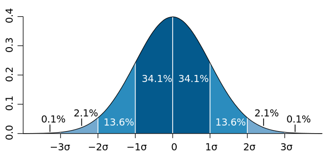
For example, knowing that 34.1% of our data will be within one standard deviation (\(\sigma\)) above the mean and 34.1% will be within one standard deviation below. Together, this tells us that the interval generated by \(\mu \pm \sigma\) should contain about 68.2% of the total observations. That is,
\[ (\mu - \sigma, \mu + \sigma) = \text{interval with 68.2% of data} \] As our sampling distribution is approximately normal, we can approximate this interval with the statistics generated from our sample mean:
\[ (\overline{x} - \hat{\sigma}, \overline{x} + \hat{\sigma}) \approx \text{interval with 68.2% of data} \]
Fortunately, this process also works in reverse: once we have determined the probability we want for our interval to contain the true value, we can work backwards to find the appropriate values. A common interval size used in statistics is to capture the true mean with a probability of 95%, also called a 95% confidence interval. The probability itself, in this case 95%, is known as the coverage probability. For the normal distribution, a 95% coverage probability is given with the interval \(\overline{x} \pm 1.96 \hat{\sigma}\). It is important to note here that, just like the normal distribution itself, the confidence interval is also symmetric around the mean.
Of course, other values can be used, generating confidence intervals of different sizes. To introduce this more general case (that is, without specifying a value), we need a few variables in the previous example. Let’s begin with coverage probability. We use the value \(1 - \alpha\) to describe the coverage probability, where \(\alpha\) represents the probability that our interval does not contain the true mean. This may seem a bit backwards at first, but our reasons for doing so will be clear shortly.
If \(1 - \alpha\) represents our coverage probability, then \(\alpha\) must represent the probability of our interval not containing the true value. And, as our interval is symmetric about the sample mean, this means that there is a probability of \(\alpha/2\) that the true value is outside of our interval and above the sample mean, while a probability of \(\alpha/2\) that it lies outside of our confidence interval and below the sample mean. This concept is illustrated below:
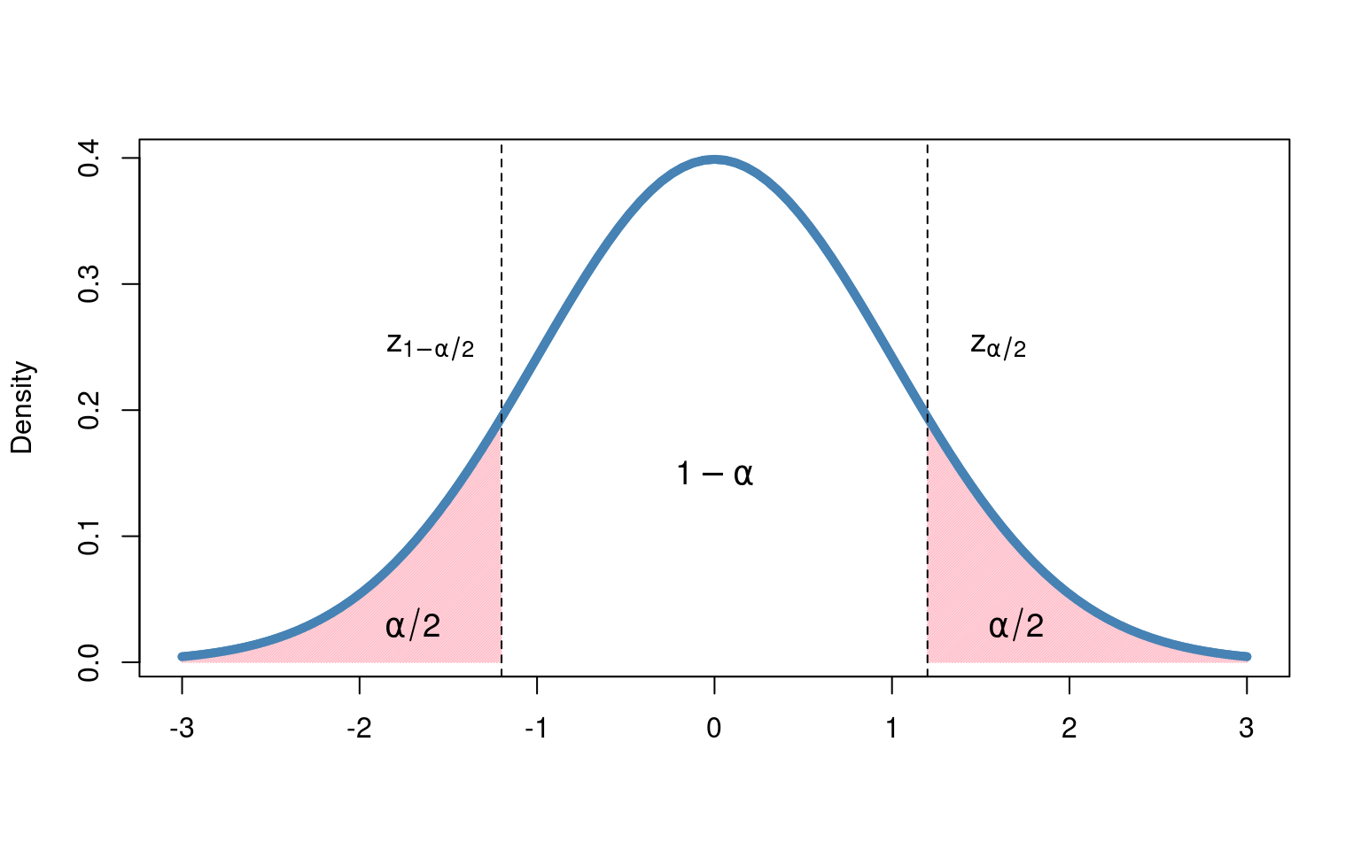
As you may have guessed, the lines at \(z_{1-\alpha/2}\) and \(z_{\alpha/2}\) represent the endpoints of our confidence interval. These values are known as critical values. In particular, \(z_{1-\alpha/2}\) gives us the value for which \(\alpha/2\%\) of the distribution is less than \(z_{1-\alpha/2}\), and \(z_{\alpha/2}\) gives us the value for which \(\alpha/2\%\) is greater. In the case of a 95% confidence interval, we have that \(\alpha = 0.05\), and our critical values are denoted \(z_{0.025}\) and \(z_{0.975}\)
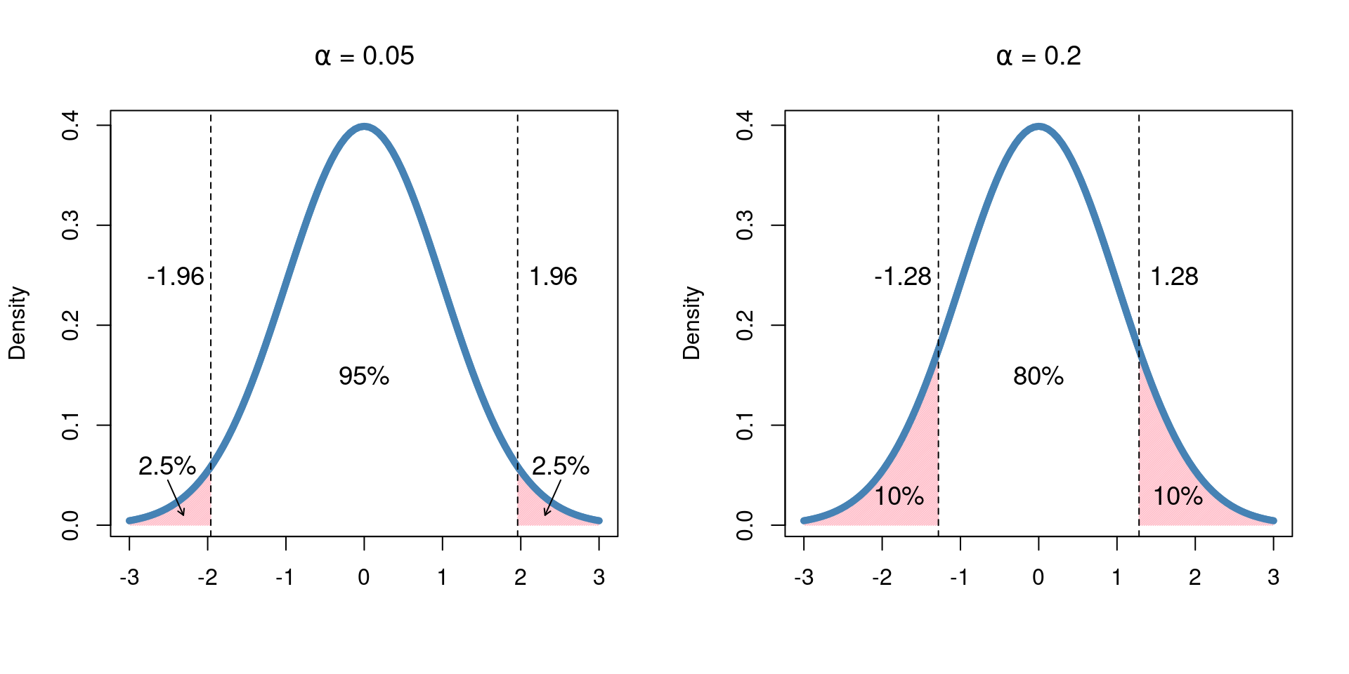
By changing the values of \(\alpha\), we are able to change the probability that our generated interval contains the true value and, as a consequence, change the size of the interval itself. We illustrate this below by considering two different commonly used values for \(\alpha\) and the intervals that are generated:
The mathematical details of constructing a confidence interval depends on the parameter of interest and how the study was designed. Here, however, we will focus on conceptual understanding and interpretation, using sample data and sampling distributions to construct our \(100(1-\alpha)\)% confidence intervals.
Before moving on, let’s take a moment to review where we are and what we know:
We are interested in constructing an interval that captures a fixed but unknown quantity about our population, in this case, \(\mu\). This value is not random.
What is random, however, are the values used to construct this interval, namely \(\overline{X}\) and \(\hat{\sigma}\). These values come from our random sample and, as such, follow a sampling distribution.
In practice, we are generally only able to collect a single random sample, giving us single estimates of \(\overline{X}\) and \(\hat{\sigma}\) and, consequently, a single confidence interval.
An important question to ask ourselves at this point is: If there is a single true parameter whose value we do not know, and if we can only construct a single confidence interval from our sample data, what does it mean for a confidence interval to have a coverage probability of 95%?
The answer to this lies in the sampling process itself. Specifically, what we mean when we say that an interval has a coverage probability of 95% is:
If we were to continuously collect samples from our population in the exact same way and
for each sample, we compute the sample mean and standard error and
use these values to construct our confidence interval then
95% of the time, our computed confidence interval will contain the true parameter value.
In other words, although we will never know for certain if our particular interval contains the true value, we can take confidence (see what we did there?) in knowing that the process will give us a valid interval 95% of the time. Let’s explore this concept a little further by playing with the following applet.
Exercise 7.2
The applet below is designed to help you get familiar with some of the important concepts related to confidence intervals. The inputs to the simulation are the sample size, number of experiments, and the confidence level. The simulation proceeds by taking a sample of the specified size and constructing a confidence interval based on that sample with the specified level of confidence. This process is one experiment. Each sample is drawn from the same population. For a specified number of experiments, the sampling and confidence interval construction is repeated either 10, 50, 100, or 1000 times. The plot shows all the confidence intervals constructed from each experiment – the number of intervals shown is equal to the “Number of Experiments.” The true population parameter in this case is 0 (only for simplicity). Intervals are shaded in blue if they cover the true population parameter and red if they do not contain the true parameter. The applet also reports the “observed coverage” from all experiments, this is the proportion of all the intervals shown that did contain the truth. Clicking “Run Simulation” will redo the specified number of experiments using the inputs provided.
-
Set the sample size to 30, the confidence level to 95%,
and simulate running 100 experiments (100 intervals total).
- How many intervals did not contain the true population parameter? In other words, how many red intervals are there?
- What was the observed coverage? Show how this was computed based on the number of intervals that did/did not contain the truth.
- Given the specifications use, What would you expect the coverage to be?
- Re-run the simulation under the same conditions (click “Run Simulation” again). What was the observed coverage for the second set of 100 experiments?
- Did you get the same observed coverage for both simulations? What does this indicates about the simulation?
- Re-run the simulation several times and compare the observed coverage from each run. What do you notice?
-
Keep the confidence level at 95%, but change the sample size to 50. Simulate 100 experiments.
- How do the intervals differ from those constructed from experiments using a sample size of 30?
- What is the observed coverage? What would you expect the coverage to be based on the specifications used?
- Across the 100 confidence intervals shown, how do the widths of the confidence intervals compare? Is there any difference in the confidence interval widths between intervals that do contain the true parameter and those that do not?
- Now change the sample size to 100. How do these intervals compare to those using sample sizes of 30 or 50? Does the sample size seem to impact the coverage probability?
- Change the confidence level to 50% and again run several simulations with sample sizes of 30, 50, or 100. How do these compare to other simulations we have seen? What appears to be the relationship between sample size, the confidence level, and the width of the intervals?
-
Return to a sample size of 30 and set the number of experiments to be 1000.
- Run the simulation once with a confidence level of 95%. What is the observed coverage?
- Re-run the simulation several more times with 1000 experiments each. What are the coverage probabilities? How do these compare to (f) in question 1?
- Re-run the simulation using a confidence level of 50%. How do these intervals compare to those using a confidence level of 95%? How does this change with different sample sizes?
-
Change the parameters of the simulations as needed to answer the following true/false questions. Explain your answers.
- As the sample size increases, the coverage probability increases.
- As the confidence level decreases, the width of the confidence intervals decreases,
- As the sample size increases, the width of the confidence intervals increases.
- If a researcher wants a narrower confidence interval, they should obtain a larger sample.
- If a researcher wants a wider confidence interval, they should increase the confidence level.
Definition 7.1
Point Estimation: Using a single numeric quantity to estimate a population parameter
Interval Estimation: Using a range of numeric values to estimate a population parameter
Coverage Probability: The probability that a constructed confidence interval contains the true population parameter
Critical Value: The cutoff value that defines the upper and lower bounds of a confidence interval interval
Confidence Interval: An interval estimate which contains the true population parameter according to a specified confidence level
7.3 Hypothesis Tests
Often, the motivation for performing a particular experiment is to answer a scientific question about a population. We have just seen that, along with the CLT, the collection of a sample mean along with a standard error allows us to construct an intervals of values representing likely values of the true parameter.
Along with parameter estimation, a cornerstone of statistical inference is significance testing. Confidence intervals allow us to construct a range of plausible values for the parameter, and significance tests allow us to determine the likelihood of a parameter taking a certain value. A hypothesis test uses sample data to assess the plausibility of each of two competing hypotheses regarding an unknown parameter (or set of parameters). A statistical hypothesis is a statement or claim about an unknown parameter. The null hypothesis generally represents what is assumed to be true before the experiment is conducted. This hypothesis is typically denoted \(H_0\). The alternative hypothesis represents what the investigator is interested in establishing; this hypothesis is typically denoted \(H_A\). Oftentimes when people refer to the “scientific hypothesis,” this in reference to the alternative hypothesis – it is what the investigators think will happen or what they want to show. The goal of a hypothesis test is to determine which hypothesis is the most plausible – the null or the alternative.
As an example, consider researchers that have developed a new drug to treat cancer. In order for the drug to be approved for use, the investigators must prove that it is more effective in treating cancer than the current treatment options. To do this, the investigators gather a sample of cancer patients and randomize half of them to receive their new drug and half to receive the current treatment. Then they determine how many patients improved in both groups. In this scenario, the null hypothesis would be that the new drug and the current drug result in the same improvement. Why? Well, the null hypothesis is what is believed before the data was collected. The key is whose beliefs we are talking about. While the scientists that developed the drug most likely believe that their new drug is more effective, the rest of the scientific community remains in a state of uncertainty. The null hypothesis reflects the general beliefs of the scientific community. The alternative hypothesis in this scenario is that the drugs differ in their effectiveness on treating cancer.
In general, we can think about the null hypothesis as being the “baseline,” “boring,” “nothing to see here” hypothesis. The exact specification will depend on the study context and the type of data being measured (categorical or continuous):
- \(H_0\): the average cholesterol for hypertensive smokers’ is no different than the general population
- \(H_0\): no difference between the treatment and control groups
- \(H_0\): men and women have identical probabilities of colorectal cancer
- \(H_0\): observing a “success” in a population is identical to flipping a coin
The hypothesis testing procedure uses probability to quantify the amount of evidence against the null hypothesis. Since the null hypothesis is the baseline, we start by assuming that it is true. Then, we conduct the study and collect data to quantify the likelihood that the the null is true. The reason for this approach is rooted in the scientific method. As we introduced in Chapter 1, the scientific method has 7 steps:
- Ask a question
- Do background research
- Construct a hypothesis
- Test your hypothesis with a study or an experiment
- Analyze data and draw conclusions
- How do the results align with your hypothesis?
- Communicate results
We are really focusing on steps 3-5. In step 3, we construct the “scientific hypothesis” and in step 4, we test that hypothesis. In order to produce rigorous scientific results, we cannot assume that the scientific hypothesis is true, as that is the goal of our study. We must assume the current state of knowledge (null hypothesis), and then if we are to prove that our hypothesis is correct, we would show that if the current knowledge was true, it would be really unlikely that our experiment would have ended up how it did.
A great analogy to the concept of hypothesis testing is our judicial system. In court, the legal principle is that everyone is “innocent until proven guilty” and the prosecution must prove that the accused is guilty beyond a reasonable doubt. In many cases, there may not be definitive evidence if the defendant is actually innocent or guilty. But, if the prosecution can show that the likelihood of the accused individual being guilty is high (or equivalently, that the likelihood of the accused individual being innocent is low), then the defendant will be convicted. In hypothesis testing, researchers are like the prosecution and must use data to prove that the null hypothesis (current state of knowledge) is false beyond a reasonable doubt. The next several chapters will go through how we can use different types of data to quantify our evidence against the null hypothesis.
With this set up in mind, we have two possible outcomes of a hypothesis test. Either we conclude that we do not have a lot of evidence against the null hypothesis, i.e. the null hypothesis looks reasonable, and we fail to reject the null or we conclude that we have enough evidence against the null and we reject the null. It is extremely important to note here that we NEVER accept the null or accept the alternative. Many people find this annoying because we can never say anything with 100% certainty. But this is exactly the point! Remember that statistics is all about quantifying our uncertainty. Think back to our drug development example. There will never ever ever be a drug that works exactly the same in every person that takes it. People are too variable, and many aspects of a person’s life impacts how a drug works in their body. It would be completely unreasonable to say that a new drug works all the time. However, there can be a drug that improves outcomes for the average person or that this drug is likely to improve outcomes in a randomly selected person who takes it.
We can create a two by two table for the results of any hypothesis test. In the rows we have the two possible outcomes from our test - fail to reject \(H_0\) and reject \(H_0\). In the columns we have the true underlying state of nature - either \(H_0\) is true or false.
| \(H_0\) true | \(H_0\) false | |
|---|---|---|
| Fail to reject \(H_0\) | Correct (1 - \(\alpha\)) | Incorrect (\(\beta\)) |
| Reject \(H_0\) | Incorrect \(\alpha\) | Correct (1 - \(\beta\)) |
In the upper-left and bottom-right cells of the table we are making the correct decision based on our test. When the null hypothesis is true, failing to reject \(H_0\) is the correct decision and when the null hypothesis is false, rejecting \(H_0\) is the correct decision. However, the other two cells correspond to a mistake being made. Because statisticians are not creative, these mistakes are referred to as type 1 error and type 2 error. A type 1 error is equivalent to a false alarm or a false positive - the null hypothesis was rejected, when in fact it was true. A type 2 error can be thought of as a missed opportunity or a false negative - the null hypothesis was false, but it was not rejected. Typically, the type 1 error rate is symbolically denoted with \(\alpha\) and the type 2 error rate is denoted by \(\beta\) (again the statisticians of the past were not creative).
If we were looking to create a good hypothesis test, we would want to minimize type 1 and type 2 errors. In other words, if we were to conduct our study over and over again and there was something to be found, we would want to reject the null hypothesis (find something) at a high rate and fail to reject the null hypothesis at a low rate. If there was truly nothing to be found, we wouldn’t want to find anything, and if there is something to be found we want to find it. However, there is a trade-off between type 1 and type 2 error. Let us illustrate this point with a simulation.
Exercise 7.3
In this experiment, we are looking to determine if a coin is fair, i.e. whether or not the probability of heads is 50%. A type 1 error in this context would be concluding that the coin is not fair, when it actually is. A type 2 error in this context would be concluding that the coin is fair when it is actually not. Each experiment consists of flipping a coin 20 times and observing the proportion of the 20 flips that result in heads. If the coin is fair, we would expect around 10 of the 20 flip to result in heads. However, if we observed 11 or 12 heads in one experiment, would you be convinced the coin isn’t fair? What about if you observed 19/20 of the flips resulting in heads?
This applet allows the user to specify the “Rejection Threshold” to determine the cutoff where the app will reject the null hypothesis. This is specified in terms of how far off the proportion of heads in the experiment is from 50%. Since we have no way to determine if the coin is more prone to heads or tails, we consider this distance in both directions. If the observed proportion of the 20 flips that result in heads is beyond the specified threshold, the null hypothesis will be rejected. For example, if you choose a threshold of 10%, then any experiment where there are 60% (12/20) or more flips resulting in heads or 40% (8/20) or less flips resulting in heads, then the null hypothesis is rejected and the coin is determined to not be fair.
The simulation involves replicating the 20 flip experiment 10,000 times. For each experiment, a coin is flipped 20 times and the proportion of heads is calculated. If that proportion exceeds the specified threshold it is counted as “Reject.” If the proportion does not exceed the threshold, that experiment is considered a “Fail to Reject.” The bar chart shows the proportion of 10,000 experiments in which the null hypothesis was and was not rejected. Note: Since we are replicating the experiment 10,000 times, we don’t expect the results to change much if the simulation is re-ran. However, you may see small changes in the proportion of rejects/fail to rejects for the same input values.
-
Set the true status of the coin to be fair and start with a threshold of 5%.
- In this setting, if we reject the null hypothesis are we making the correct conclusion or the incorrect conclusion? Explain.
- At this threshold, how many heads would cause an experiment to reject the null hypothesis
- At this threshold, what proportion of the experiments resulted in the null hypothesis being rejected?
- In terms of \(\alpha\) and \(\beta\) as described above, which of those two can you specify under these circumstances (i.e., with the true status of the coin being fair and the threshold of 5%)? What is it’s value?
- As the threshold increases, what happens to the proportion of experiments in which the null hypothesis is rejected
- Did we investigate type 1 or type 2 errors in this problem?
-
Now change the true status of the coin to be unfair with a 70% chance of heads and set the rejection threshold to 15%.
- In this setting, if we reject the null hypothesis are we making the correct conclusion or the incorrect conclusion? Explain.
- At this threshold, how many heads would cause an experiment to reject the null hypothesis
- At this threshold, what proportion of the experiments resulted in the null hypothesis not being rejected?
- In terms of \(\alpha\) and \(\beta\) as described above, which of those two can you specify under these circumstances (i.e., with the true status of the coin being fair and the threshold of 5%)? What is it’s value?
- As the threshold increases, what happens to the proportion of experiments in which the null hypothesis is rejected? Explain why.
- Did we investigate type 1 or type 2 errors in this problem?
-
Now change the true status of the coin to be unfair with a 20% chance of heads and set the rejection threshold to 20%
- In this setting, if we reject the null hypothesis are we making the correct conclusion or the incorrect conclusion? Explain.
- At this threshold, how many heads would cause an experiment to reject the null hypothesis
- At this threshold, what proportion of the experiments resulted in the null hypothesis not being rejected?
- In terms of \(\alpha\) and \(\beta\) as described above, which of those two can you specify under these circumstances (i.e., with the true status of the coin being fair and the threshold of 5%)? What is it’s value?
- As the threshold increases, what happens to the proportion of experiments in which the null hypothesis is rejected?
- Did we investigate Type 1 or Type 2 errors in this problem?
- What can you conclude about the relationship between type 1 and type 2 errors?
Definition 7.2
Hypothesis test: A decision making technique which assesses the plausibility of two competing hypotheses
Statistical hypothesis: A statement about the value of an unknown parameter
Null hypothesis: The assumed state of truth prior to running the experiment, denoted \(H_0\)
Alternative hypothesis: Range of values for the parameter we might believe are true, denoted \(H_A\)
Type I error: Rejecting a true null hypothesis, i.e., false positive
Type II error: Failing to reject a false null hypothesis i.e., false negative
7.4 P-values
All hypothesis tests are based on quantifying the probability of the study results assuming the null hypothesis is true. This probability is so important that it has a special name, the p-value. In technical terms, the p-value gives the probability of obtaining results as extreme or more extreme than the ones observed in the sample, given that the null hypothesis is true. A less technical way to describe a p-value is that assuming there is truly nothing going on, how likely are we to have seen what we have seen?
If we are thinking about hypothesis testing as a court case, p-values are the way that we can quantify the evidence against the defendant. Recall, the prosecution wants to prove beyond a reasonable doubt that the defendant is not innocent. So what does the scientific community consider sufficient evidence? There is a generally agreed-upon scale for interpreting p-values with regards to the strength of evidence that they represent.
| p-value | Evidence against null |
|---|---|
| 0.1 | Borderline |
| 0.05 | Moderate |
| 0.025 | Substantial |
| 0.01 | Strong |
| 0.001 | Overwhelming |
Often, the term “statistically significant” is used to describe p-values below 0.05, possibly with a descriptive modifier.
- “Borderline significant” (p < 0.1)
- “Highly significant” (p < 0.01)
However, don’t let these clearly arbitrary cutoffs distract you from the main idea that p-values represent – how far off is the data from what you would expect under the null hypothesis. A p-value of 0.04 and 0.000000001 are not at all the same thing, even though both are “statistically significant.”
In general, a type I error rate, \(\alpha\), is chosen prior to beginning the study. That is, investigators specify beforehand how much evidence should be needed to reject the null hypothesis. The smaller the value of \(\alpha\), the greater the “burden of proof” required. If the observed p-value is smaller than the specified \(\alpha\), the null is rejected. In the context of rejecting or failing to reject a hypothesis, \(\alpha\) is also commonly referred to as the significance level.
A fundamental property of p-values is that if we use \(p < \alpha\) as cutoff for rejecting the null hypothesis, the type I error rate is guaranteed to be no more than \(\alpha\). However, the \(p < \alpha\) cutoff guarantees us nothing about the type II error rate. This is because p-values are calculated assuming the null hypothesis is true, so they don’t give us any information about what to expect when the null hypothesis is false.
While p-values are widely used, have a distinct purpose, and can be informative they also have a number of limitations.
Definition 7.3
p-value: The probability of observing data as extreme or more extreme than what was observed in the sample, given the null hypothesis is true
Statistically significant: When the p-value is \(<\) 0.05. Not necessarily related to clinical significance
Significance level: The p-value cutoff used to determine if the null hypothesis is rejected Denoted \(\alpha\) and often considered to be 0.01, 0.05, or 0.1