Introduction to Probability Distributions
In Chapter 4, we introduced the idea of random processes, i.e. situations
in which the outcome can not be determined perfectly in advance. Random processes
are defined in terms of the collection of possible events (sample space) and their
associated probabilities. In that chapter, we saw three methods for calculating
probabilities – the enumeration method, the probability function method, and the
simulation method. In this chapter we will expand on the probability function
method, which uses a known function called a probability distribution to
determine the probability of each event.
Probability distributions are closely related to random variables, numeric
variables that can take on different values depending on the outcome of a random
process. In previous mathematics courses you may have seen variables such as
\(x\) or \(y\) used as placeholder values which are then solved for. For example,
you can solve for the variable \(x\) in \(4x + 5 = 25\), to determine \(x = 5\). By
contrast, the outcome of a random variable is not be predetermined. Instead,
we talk probabilistically about the likelihood of observing each possible outcome.
Random variables are typically denoted with capital letters, e.g., \(X\) or \(Y\),
whereas the observed outcome of the random process is denoted with lowercase letters
\(x\) or \(y\). For example, flipping a coin three times is a random process. We can
define the random variable \(X\) to represent the number of heads we observe
between the three flips. \(X\) can take on four possible values: 0, 1, 2, or 3. If
we observe 2 heads, we have \(x = 2\).
Most simply, a probability distribution (often just called a distribution)
is a method for taking a possible event as input and giving us the corresponding
probability as output; the corresponding probability tells us how likely it is
that the specific event will occur, out of all of the possible events. We often
say random variables have or follow a probability distribution, as the
distribution quantifies the probability of observing the possible values a random
variable can take on. We can denote a probability distribution as \(P(X = x)\), or
the probability that the random variable, \(X\), takes on a generic value, \(x\).
There are many useful probability distributions that have
been defined by mathematicians and statisticians to describe a variety of scenarios:
Counting the number of successes in a fixed number of trials that can results
in either success or failure, such as counting the number of heads when flipping a
coin three times
Counting the number of successes before the first failure in a series of
success/failure trials, such as counting the number of days before a light bulb
burns out
Describing the length of time between events that occur at a constant rate, such
as the time between phone calls at a help desk
Describing range of continues values, such as the blood pressure in adults
One can represent a probability distribution visually using a probability histogram.
On the x-axis, we have the possible outcomes of the random process – the values
the random variable could take. For each outcome, the bar height represents
the probability of observing that value. For the coin flipping example, the
probabilities of observing each possible number of heads can be represented as:
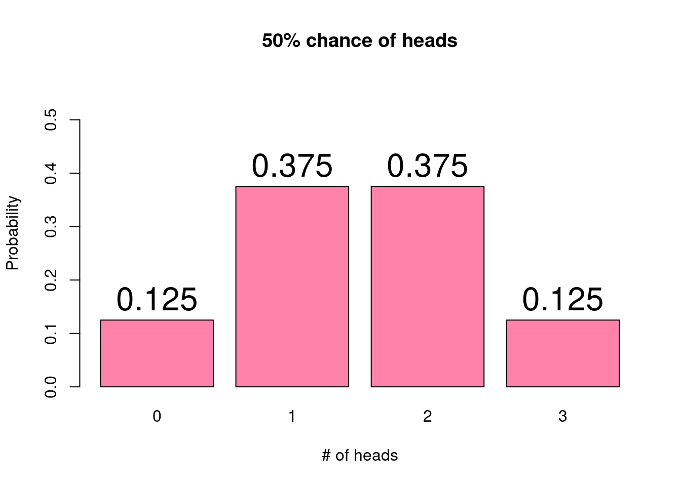
When looking at a probability histogram, we can characterize the shape of the
distribution analogously to how we talk about a histogram of observed data. We
often use unimodal distributions, which may or may not be skewed. For example,
the above probability histogram shows a unimodal and symmetric distribution.
The beauty of using probability distributions to describe the likelihood of all
outcomes of a random process is its simplicity. Probability distributions rely
on a small number of parameters which determine the distribution’s shape. In
the coin flipping example, we could consider one of the parameters to be the
probability of obtaining heads. We assume that we have a fair coin and that this
probability is 50%. If instead we had a weighted coin with a 60% chance of
landing on heads, the probability distribution would change. That is, the probability
associated with each possible outcome would be different.
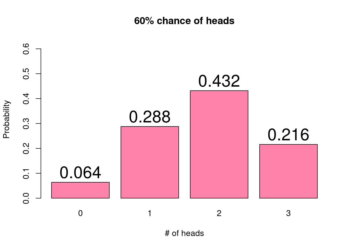
With a higher chance of the coin resulting in heads, we now see that the three
flips are more likely to result in 2 or 3 heads and much less likely to result
in 0 heads. In other words, the distribution is now slightly skewed left.
Because these probabilities can be described by a distribution function, we can
easily compute and compare the probabilities of each possible outcome as a function
of the distribution parameter, in this case, the probability of flipping heads.
Another key concept related to probability distributions and random variables is
the idea of the expected value, often denoted \(E(X)\). The expected value of a random variable, often
denoted as \(E(X)\), is a weighted average which provides a measure of the central
mass of the probability distribution. The expected value averages over all possible
outcomes of the random variable with each outcome weighted according to its
probability. We can also think of the expected value of a random variable as its average
value. In more technical terms, we might say that the expected value is a weighted
average which provides a measure of the central mass of the probability distribution,
averaging over all possible outcomes of the random variable with each outcome weighted
according to its probability. Whew!
Returning to the coin flipping example with a fair coin, we have
seen that the probability distribution is:
|
x
|
P(X = x)
|
|
0
|
0.125
|
|
1
|
0.375
|
|
2
|
0.375
|
|
3
|
0.125
|
Multiplying each possible outcome (\(x\)) by its associated probability (\(P(X=x)\))
and adding them together (which happens to be the definition of a weighted average)
gives us an expected value of
\[(0 \times 0.125) + (1 \times 0.375) + (2 \times 0.375) + (3 \times 0.125) = 1.5.\]
Looking at the probability histogram, this value should make sense as it falls
right in the center of the distribution.
Expected values are more easily conceptualized in terms of a game or bet. For
example, consider the following game: you flip a fair coin; if the coin lands on
heads, you win $20, and if the coin lands on tails, you lose $1. Would you play
this game? Assuming you have a spare dollar, the answer is probably yes. Since
you have equal chances of the coin landing on heads or tails, you are just as
likely to win $20 as you are to lose $1. In terms of the expected value, it
would be
\[(20 \times 0.5) + (-1 \times 0.5) = 9.5.\]
The expected value tells us that if you were to play this game over and over,
you would be expected to win $9.5 per game. Critically, it is worth reiterating
here that for any single instance of this game, you can only win $20 or
lose $1. The $9.50 indicates the long term average over many games.
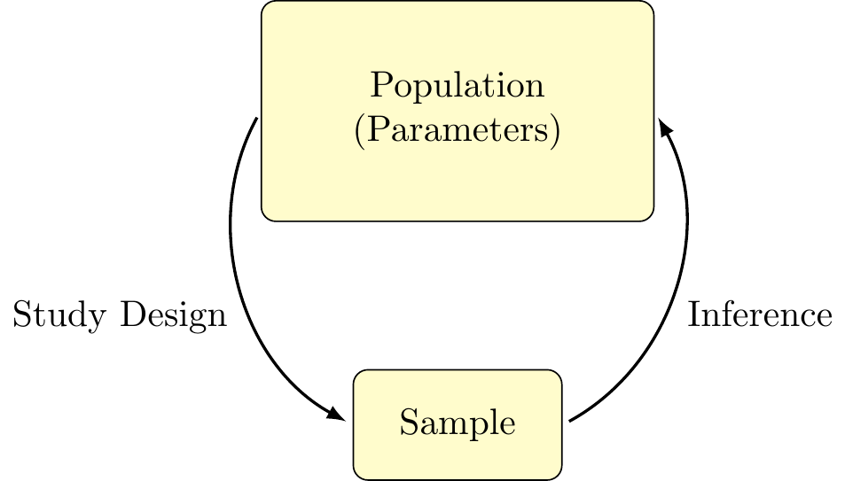
Finally, let’s discuss how probability distributions relate back to our general
statistical framework. In our framework, we are interested in learning about the
population, which we assume follows some probability distribution. This distribution
is governed by a set of unknown parameters. When we collect a sample, we expect
that the distribution of the sample will be similar to that of the true population.
As we will see in the following chapters, our sample will be used to compute statistics,
or estimates of the true parameters. Indeed, much of statistical inference involves
estimating the values of these parameters, with associated measures of certainty.
We end this chapter with a discussion of two of the most commonly used distributions,
the binomial and the normal.
Probability distribution: A method for assigning probabilities to all possible events
Random variable: A numeric variable whose value depends on the outcome of a random process
Probability histogram: A graphical display of a probability distribution
Parameters: Values associated with a probability distribution that determine the distributions shape
Expected value: The weighted average of the outcomes of a random variable, with weights determined by their probability
Statistics: Values computed from a sample that serve as estimates of the
population parameters
Binomial Distribution
The first distribution we will examine in depth is the binomial distribution,
describing the number of successes in a fixed number of independent trials
that can result in one of two outcomes (success or failure), where the probability
of success is the same between trials. As the data from a binomial distribution
fall into distinct categories, the binomial distribution is also a member of a category
of distributions known as discrete distributions.
We have already seen one example of the binomial distribution in detail – flipping
a coin some number of times and counting the number of flips result in heads (success).
Each flip has two possible outcomes (heads or tails), the same probability of heads
on each flip (50%), and a predetermined the number of trials (three flips).
To illustrate another example of the binomial distribution, we might consider
rolling a six-sided die a number of times, counting the number of rolls that result
in either a 5 or 6. That is, we would consider a success to be rolling a 5 or 6, and
a failure to be rolling a 1, 2, 3, or 4. As there are six equally likely outcomes,
with two of these being considered a success, we note that for any particular roll
(trial), the probability of success is 2/6, or 1/3. The takeaway here is that, even
though there are six possible values for a given roll, we can still posit a binary
outcome and determine the associated probabilities.
As you may have noticed from these two examples, the binomial distribution
can be used for various success probabilities and numbers of trials. In fact,
these quantities define the two parameters of the binomial distribution. These
parameters are typically denoted as \(n\), the number of trials, and \(p\), the probability of
success. The binomial distribution can be written as a function of these parameters:
\[
P(X = x) = \binom{n}{x} p^x (1-p)^{n-x}.
\]
While this may look like a nasty formula, don’t be afraid! Probabilities following
a binomial distribution can be easily computed by any statistical software. For
this reason, we will focus on the distribution properties rather than performing
calculations.
For any valid value of \(n\) and \(p\), we can use the binomial distribution
to compute the probability of observing any possible outcome. Valid values of \(n\)
and \(p\) simply mean that the number of trials conducted must be a positive integer
(e.g., 1, 2, 3, …) and that \(p\) must be between 0 and 1 (it is a probability after all).
The expected value of the binomial distribution is given by \(E(X) = n \times p\), or
the total number of trials times the probability of success for each trial. To gain
a better understanding of how these parameters impact the shape of the distribution,
we will use the following applet.
The applet below is designed to help you get familiar with the parameters of the
binomial distribution, and how they impact the probability distribution.
You can change the values of the number of trials \(n\), and
the probability of success \(p\), and the app will display the associated distribution
in a probability histogram.
Use the applet to answer the following questions:
Set \(n = 10\), and change the value of \(p\) (note: you can press the triangular
“play” button to have the app vary \(p\) automatically). What happens to the shape of the
distribution as \(p\) gets closer to 0? What about when \(p\) gets closer to 1?
Now, set \(p = 0.4\) and vary \(n\) over the range of possible inputs. What do
you notice about the x-axis as \(n\) is changing? Explain this trend by referring
back to what \(n\) represents.
Keeping \(p\) constant and varying \(n\) between 20 - 50, does the shape of the
distribution change? What about the location of the distribution?
The applet below is designed to familiarize you with data generated from the
binomial distribution. That is, we are interested in exploring the relationship between an underlying theoretical distribution and data that is observed. You can change the values of the number of trials \(n\), and
the probability of success \(p\) to specify the parameters of the population
distribution. Then, you can take a random sample from the distribution.
Use the applet to answer the following questions:
Set \(n = 10\) and \(p = 0.5\). Starting with a sample size of 10, simulate data a number of times and observe the histogram of the observed data. What do you notice? Is the observed data typically centered around the same value as the probability distribution? Does it have the same shape? Try again with a sample size of 50. What has changed? What stays the same? Do this once more with a sample size of 100.
What are some general observations that can be made from the results in saw in (1)? How consistently does a histogram of the observed data match that from the theoretical distribution? What effect does sample size have on this consistency?
Play around with different values of \(n\) and \(p\), as well as with different sample sizes. What are some trends that you notice? Are there values of \(n\) and \(p\) that seem to produce more consistent results? If you were to only look at the observed data, how confident do you feel that you could guess the shape of the underlying distribution? How close might you be?
In general, how would you describe the histogram of the binomial distribution? Does it tend to be symmetric? How do different values of \(p\) change the skew of the distribution? How about different values of \(n\)?
Binomial Distribution: A probability distribution that characterizes the
probabilities of observing some number of successes in a fixed number of
trials, each with two possible outcomes and the same probability of success
Discrete Distribution: Any probability distribution that depicts the
occurrence of distinct, countable values
Normal Distribution
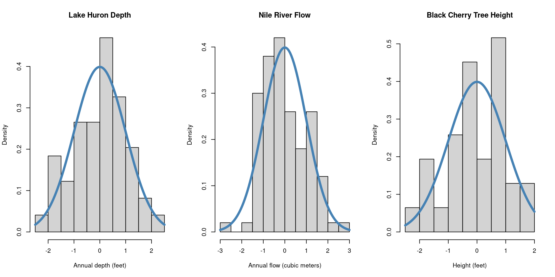
Let’s begin by considering three histograms, each describing a set of continuous
data collected from various sources. First, we have the annual depth of Lake Huron
from 1875-1972 measured in feet. Next, the annual flow of the river Nile from 1871-1970
measured in cubic meters, and lastly, the recorded height, in feet, of 31 black cherry
trees. What do all of these histograms seem to have in common?
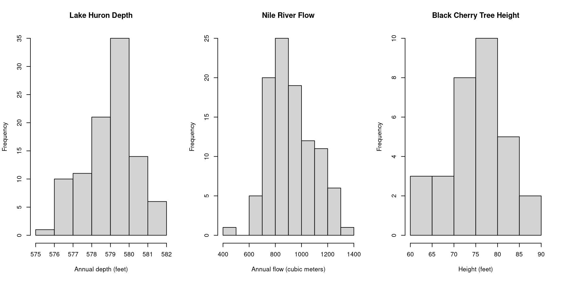
What we see here are examples of a normal distribution (also known as a bell curve),
one of the most ubiquitous distributions in all of statistics. The normal distribution
is characterized by the “bell shape” that is symmetric about it’s center.
Like the binomial, the normal distribution is characterized by two parameters,
\(\mu\) and \(\sigma^2\), representing the mean and the variance, respectively. The
mean value, \(\mu\), indicates the location of the peak on the x-axis, whereas the
variance, \(\sigma^2\), indicates the amount of dispersion about the mean. A random
variable \(X\) that follows a normal distribution can be expressed \(X \sim N(\mu, \sigma^2)\),
or, “The random variable \(X\) follows a normal distribution with mean \(\mu\) and
variance \(\sigma^2\).” The formula for the normal distribution is given as
\[
\begin{align*}
f(x) = \frac{1}{\sqrt{2 \pi \sigma^2}} \ e^{- \frac{(x-\mu)^2}{2\sigma^2}}.
\end{align*}
\]
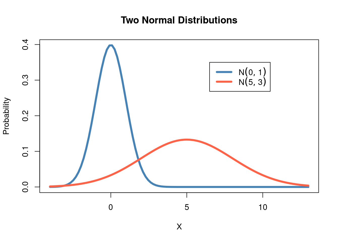
Consider the two normal distributions below, with different values for \(\mu\) and
\(\sigma^2\). Although they are centered at different locations and have different
amounts of dispersion around the mean, they are both bell-shaped curves characteristic
of the normal distribution:
Given that the normal distribution appears so frequently in statistics, it is common
practice to standardize a normal distribution so that it has a mean value of \(\mu = 0\)
and variance \(\sigma^2 = 1\) (note also that the standard deviation is
\(\sigma = \sqrt{\sigma^2} = \sqrt{1} = 1\)). A normal random variable that has been
standardized is called a standard normal distribution and is often written
\(Z \sim N(0,1)\). We can consider again the histograms above, once they’ve been
standardized:
Unlike the binomial distribution, in which there are \(n\) possible values that our
random variable can take, the normal distribution represents a random variable that
is continuous over a range of values, making the normal distribution a member
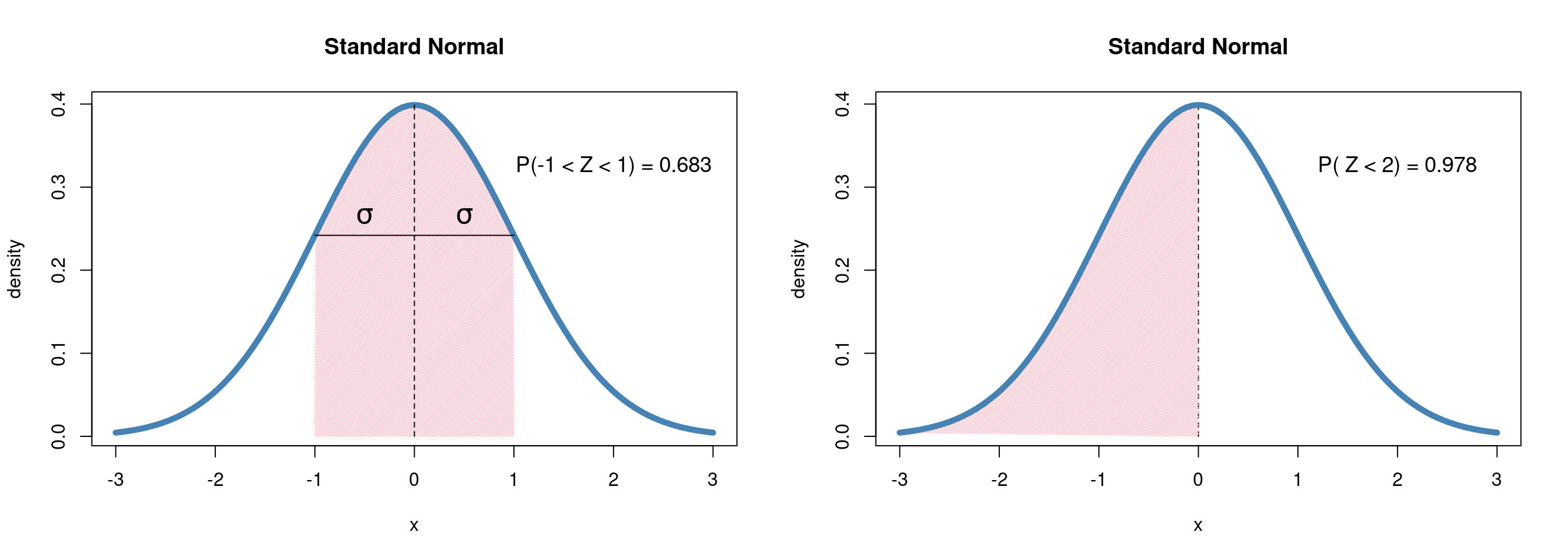
of the family of continuous distributions. Instead of asking the probability
of a specific value, say, \(Z = 0\), probabilities are given as the area under the
curve for a certain interval. We might ask, “What is the probability that \(Z\) is
one standard deviation (\(\sigma\)) away from \(0\)?” or perhaps, “What is the probability
that \(Z < 0 ?\)”
We will return to the normal distribution in the following chapters, demonstrating
both how it arises naturally in the study of statistics and the powerful toolkit
it provides in the field of statistical inference.
The applet below is designed to help you get familiar with the parameters of the
normal distribution, and how they impact the probability distribution.
You can change the values of the mean \(\mu\), and
the standard deviation \(\sigma\), and the app will display the associated distribution
in a probability histogram.
Use the applet to answer the following questions:
Start by setting \(\mu = 0\) and \(\sigma = 1\). How would you describe the shape of the distribution? Is it symmetric? How concentrated are the range of values around zero?
Now set \(\sigma = 2\). What has changed? Reset the value back to \(\sigma = 1\) and press the “Play” button. How does the normal distribution change with \(\sigma\)?
Repeat exercise 2, this time setting \(\sigma = 1\) and allowing \(\mu\) to change over a range of values. How does the distribution change? How does it change compared with what we saw in exercise 2?
Play around with different values of \(\mu\) and \(\sigma\). What impact does changing \(\mu\) have on the concentration of values? How does changing \(\sigma\) impact where the distribution is centered? How would you describe the relationship between \(\mu\) and \(\sigma\)?
Compare your answers from this exercise with those from the binomial distribution. How do these distributions differ in their relationship to their parameters?
The applet below is designed to familiarize you with data generated from the
normal distribution. You can change the values of the mean \(\mu\), and
the standard deviation \(\sigma\) to specify the parameters of the population
distribution. Then, you can take a random sample from the distribution.
Use the applet to answer the following questions:
Start again by setting \(\mu = 0\) and \(\sigma = 1\), and simulate data several times with a sample size of 10. How does the observed data compare to the probability distribution? Does it have the same shape? What changes when we set our sample size to 50?
Compared with the binomial distribution, how well does data generated from a normal distribution tend to match the probability distribution? Given only the observed data, how close do you think your estimate would be of the underlying distribution?
Normal Distribution: A continuous bell-shaped distribution with
two parameters that are the mean value, \(\mu\), with a variance \(\sigma^2\)
Standard Normal Distribution: A special case of the normal distribution,
\(Z \sim N(0, 1)\)
Continuous Distribution: Any probability distribution that depicts the
occurrence of a random variable that can take an infinite set of possible values
within a given (potentially infinite) interval